
自定义结果展示
在 FlexDMO 平台中,您可以通过自定义结果展示来在测试模块(Test module)中可视化算法的优化过程和结果。本文档将详细介绍如何实现自定义结果展示,以及如何在平台中使用它们。 如下图绿色高亮区域所示,您可以在"Result Display"区域实时查看算法的优化结果: 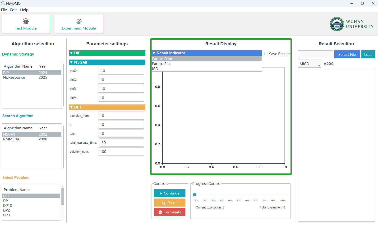
1. 注册结果展示指标
在自定义结果展示前,首先需要在 plots/test_module/config.json 文件中注册您的结果指标。 该文件用于定义平台"Result Display"区域下拉菜单中可选的结果类型。例如:
json
{
    "result_indicator": [
        "Pareto Front",
        "Pareto Set",
        "IGD",
        "Your Display..."
    ]
}- 每个字符串代表一个可供选择的结果展示类型。
- 您可以根据需要添加、修改或删除指标名称,平台会自动识别并在界面中显示。
注意: 只有在此处注册的结果类型,后续自定义展示模块才能被平台正确调用和显示。
2. 注册与实现绘图函数
注册完展示指标后,需要在 plots/test_module/draw_population.py 文件中实现对应的绘图函数。平台会根据您在 config.json 中注册的结果类型,自动调用这里的绘图方法进行结果展示。
步骤说明
定义绘图函数
在draw_population.py文件中,按照已有函数风格,添加您的自定义展示函数。例如:pythondef draw_YourDisplay(information, ax): # information: 当前优化信息 # ax: matplotlib 的轴对象 # 清除上一次绘图内容(重要!) ax.clear() # TODO: 实现您的自定义绘图逻辑 passTIP
information的详细结构说明请参见:information 数据结构说明在调度函数中注册
确保在draw_selected_chart函数中添加您的展示类型分支,例如:pythondef draw_selected_chart(information, ax, chart_type='Pareto Front'): if chart_type == 'Pareto Front': draw_PF(information, ax) elif chart_type == 'IGD': draw_IGD_curve(information, ax) elif chart_type == 'Pareto Set': draw_PS(information, ax) elif chart_type == 'Your Display...': draw_YourDisplay(information, ax) else: raise ValueError(f'未知的图表类型: {chart_type}')
3. 完整绘图函数示例
以下是平台内置的 draw_PF 函数实现,供自定义展示时参考:
python
def draw_PF(information, ax):
    # 当前时间步 & 当前评估次数
    t_now = information.get("t", '?')
    evaluate_time = information["evaluate_times"]

    # 当前种群与目标函数值
    population = information["population"]
    pf_matrix = population.get_objective_matrix()
    true_PF = information.get("POF", None)

    ax.clear()

    # --- 获取历史信息 ---
    history = global_vars['test_module'].get("runtime_populations", {})

    # 只取当前时间步之前的4个时间步
    recent_times = [t for t in history if t < t_now][-4:] if len(history) > 4 else [t for t in history if t < t_now]
    # --- 绘制历史 PF(灰色,变淡) ---
    for t_hist in recent_times:
        try:
            info_hist = history[t_hist]
            last_key, last_value = list(info_hist.items())[-1]
            pf_hist = last_value["population"].get_objective_matrix()
            pof_hist = last_value["POF"]
            if pof_hist[:, 0] is not None:
                ax.scatter(pof_hist[:, 0], pof_hist[:, 1],
                        s=10, color='gray', alpha=0.2, marker='.')
            ax.scatter(pf_hist[:, 0], pf_hist[:, 1],
                       s=6, alpha=0.2, color='gray')
        except Exception as e:
            print(f"[绘制错误] t={t_hist}, error={e}")
            continue

    # --- 当前 PF ---
    ax.scatter(pf_matrix[:, 0], pf_matrix[:, 1],
               s=10, label="Current PF", alpha=0.6, color='blue')

    # --- 当前 POF(理论) ---
    if true_PF is not None:
        ax.scatter(true_PF[:, 0], true_PF[:, 1],
                s=10, label="Current True POF", color='orange', alpha=0.9, marker='.')

    # 图标题增加 evaluate_time
    ax.set_title(f"Dynamic PF (t={t_now}, evaluations={evaluate_time})", fontsize=10)
    ax.set_xlabel("f1", fontsize=9)
    ax.set_ylabel("f2", fontsize=9)
    ax.legend(fontsize=8)
    ax.grid(True)
    plt.tight_layout()
函数详解
1. 数据获取阶段
python
t_now = information.get("t", '?')
evaluate_time = information["evaluate_times"]
population = information["population"]
pf_matrix = population.get_objective_matrix()
true_PF = information.get("POF", None)- 时间信息:获取当前时间步
t_now和评估次数evaluate_time - 种群数据:提取当前种群的目标函数矩阵
pf_matrix - 理论前沿:获取当前环境的理论帕累托前沿
true_PF(如果存在)
2. 历史数据处理
python
history = global_vars['test_module'].get("runtime_populations", {})
recent_times = [t for t in history if t < t_now][-4:] if len(history) > 4 else [t for t in history if t < t_now]- 历史获取:从全局变量中获取运行时历史数据
- 时间筛选:仅保留最近4个时间步的数据,避免图形过于拥挤
- 性能优化:限制历史数据量,提高绘图效率
3. 历史前沿绘制
python
for t_hist in recent_times:
    try:
        info_hist = history[t_hist]
        last_key, last_value = list(info_hist.items())[-1]
        pf_hist = last_value["population"].get_objective_matrix()
        pof_hist = last_value["POF"]
        # 绘制历史理论前沿和实际前沿(灰色半透明)
        ax.scatter(pof_hist[:, 0], pof_hist[:, 1], s=10, color='gray', alpha=0.2, marker='.')
        ax.scatter(pf_hist[:, 0], pf_hist[:, 1], s=6, alpha=0.2, color='gray')
    except Exception as e:
        print(f"[绘制错误] t={t_hist}, error={e}")
continue- 数据提取:从历史记录中提取每个时间步的种群和理论前沿
- 视觉层次:使用灰色半透明显示历史数据,突出当前结果
- 异常处理:确保单个时间步的错误不影响整体绘制
4. 当前结果绘制
python
# 当前种群前沿(蓝色)
ax.scatter(pf_matrix[:, 0], pf_matrix[:, 1], s=10, label="Current PF", alpha=0.6, color='blue')

# 当前理论前沿(橙色)
if true_PF is not None:
ax.scatter(true_PF[:, 0], true_PF[:, 1], s=10, label="Current True POF", color='orange', alpha=0.9, marker='.')- 当前前沿:使用蓝色显示当前算法找到的帕累托前沿
- 理论对比:用橙色点显示理论最优前沿,便于性能评估
- 图例标识:添加图例说明,便于用户理解
5. 图形美化
python
ax.set_title(f"Dynamic PF (t={t_now}, evaluations={evaluate_time})", fontsize=10)
ax.set_xlabel("f1", fontsize=9)
ax.set_ylabel("f2", fontsize=9)
ax.legend(fontsize=8)
ax.grid(True)
plt.tight_layout()- 动态标题:显示当前时间步和评估次数
- 坐标轴标签:清晰标注目标函数维度
- 网格线:提高数据读取精度
- 布局优化:自动调整图形布局
实现要点
- 错误处理:使用
try-except确保绘图稳定性 - 性能考虑:限制历史数据量,避免内存溢出
- 视觉设计:通过颜色、透明度区分不同类型的数据
- 信息完整:同时显示算法结果和理论基准
- 动态更新:每次调用
ax.clear()确保图形刷新
TIP
你可以参考该函数的结构和信息获取方式,结合自己的需求实现个性化的结果展示。